Retail Sales Forecasting¶

I. Abstract¶

In this report I will attempt extract information on economic activity in the restaurant industry throughout the year. I will do this by applying time series techniques on retail sales (in millions of dollars) of food services and drinking places. Using a Box-Jenkins methodology, I build a model and forecast with it. I find that economic activity in the restaurant industry is highest in summer months and lowest in the two months after Christmas. I conclude from my forecasts that the demand for food services and drinking places is steadily growing.

II. Introduction¶

Retail sales are one of the primary measures of consumer demand for both durable and non-durable goods. Retail sales is an important economic indicator that widely used in government, academic, and business communities to measure economic health. This dataset provides the retail sales of food services and drinking places in millions of dollars each month.

In this report, I will model and forecast retail sales to gain insight into the state of the food-service industry. I will use differencing and Box-Cox transformations to make the data stationary. Then, I will identify candidate models from the ACF/PACF of the transformed and differenced time series. I will estimate the parameters of the candidate models and select the model using AICc and performing diagnostic checking to ensure the model is a good fit. Lastly, I will forecast on the transfromed and original data using the final model.

I was able to find that retail sales is growing steadily over time. However, my forecasts were not able to account for the near 30% drop in retail sales from Covid-19 in the past few months.

My data was downloaded from https://fred.stlouisfed.org/series/RSFSDPN. My report was made through the ggplot2, ggfortify, forecast, MASS, and qpcR packages.

III. Model Building and Forecasting¶

Model Identification¶

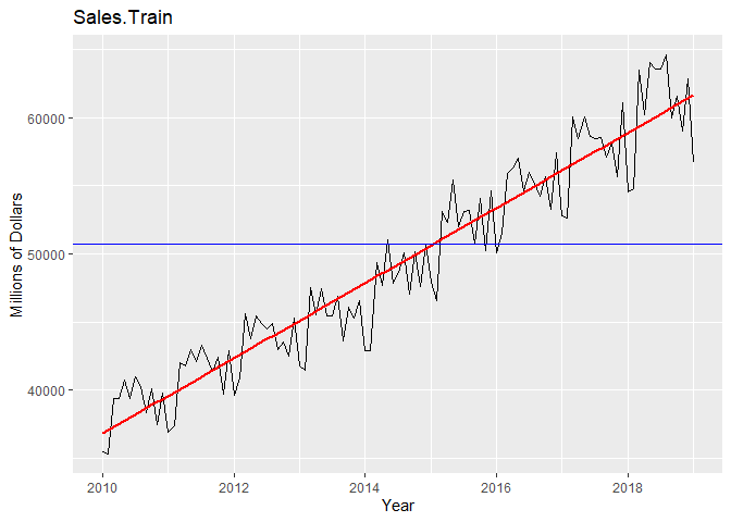
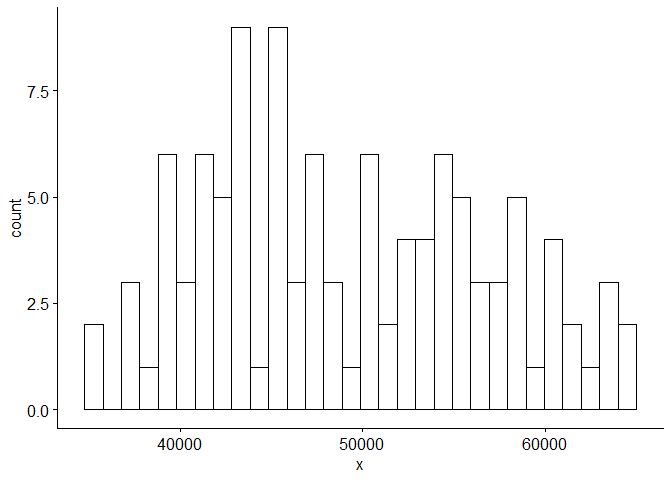
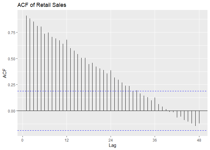
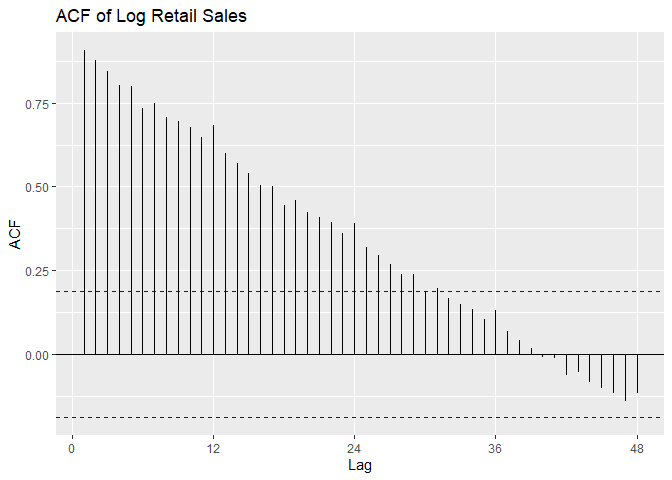
We can see from plotting the original data that the data is non-stationary: there is a linear trend and a seasonal component. The ACF confirms this as it remains large and periodic even at large lags. We suspect the period s = 12 because we see small spikes in the ACF at multiples of 12. We can also see that the variance seems to be increasing with time and the histogram of the data is skewed.

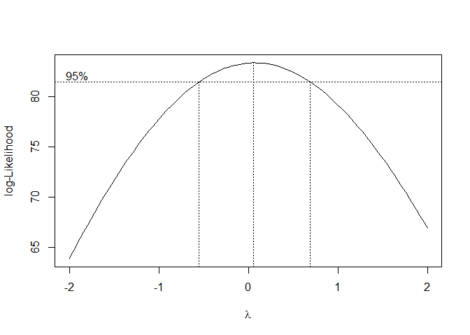
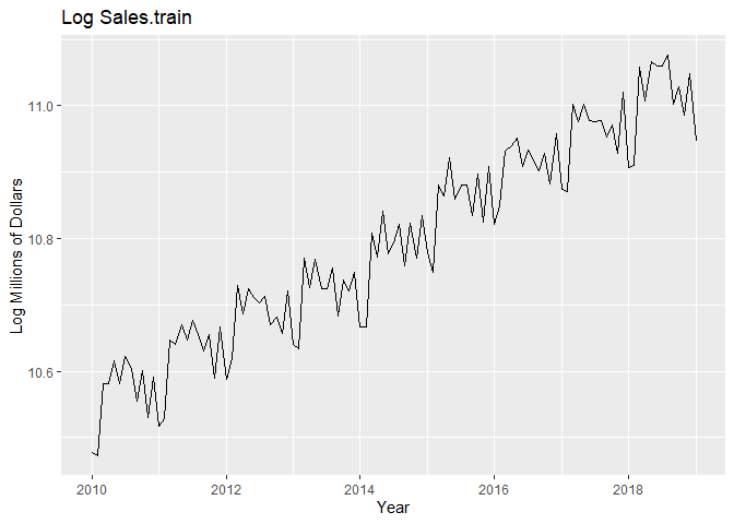
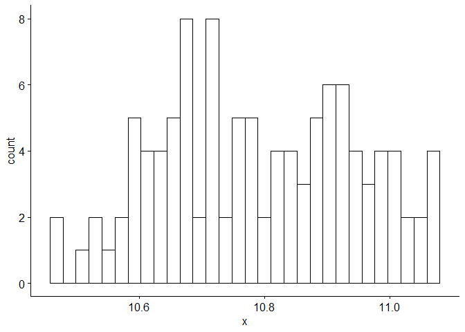
I try a Box-Cox transformation to stabilize the variance/seasonal effect and to make the data more normally distributed. Because λ = 0 is within the 95% Confidence interval of the Box-Cox transformation, we use a log-transformation on the original data. We can see that the variance is no longer increasing with time and the data is more normally distributed.

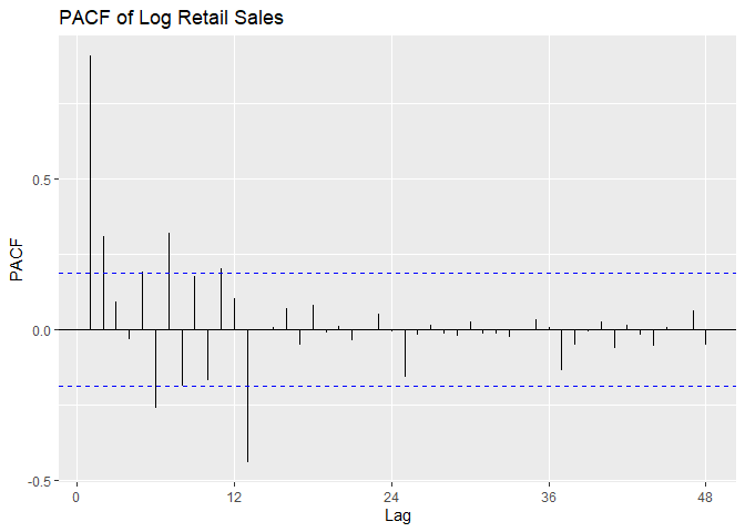
We plot the time series, a histogram, and the P/ACF of the log-transformed data here.

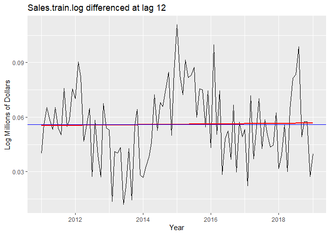
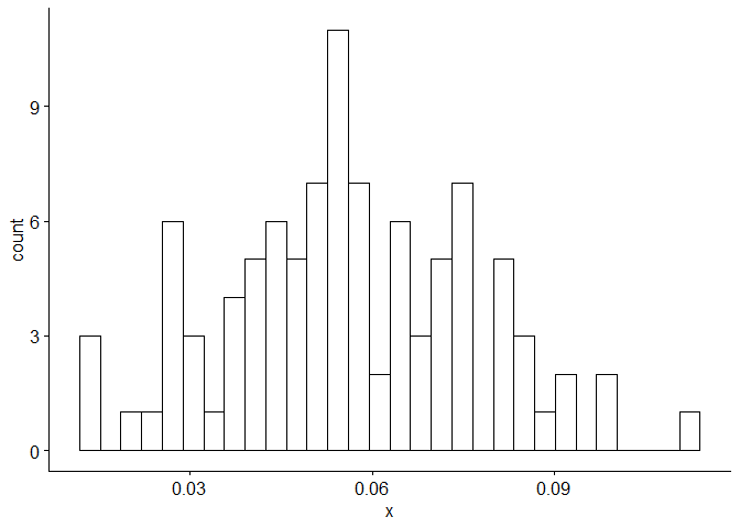
To eliminate seasonality, we try differencing the log-transformed data at lag 12. The variance decreases, so the data is not overdifferenced. From the plot we can see that there is now no trend. When we difference again at lag 1 to remove a potential linear trend, the variance increases, so the differencing is unnecessary and our data is stationary.

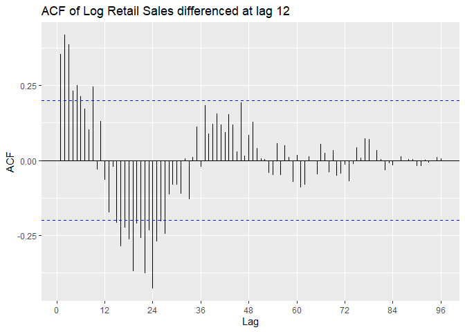
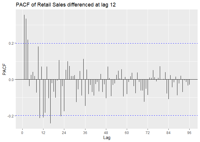
We look at the P/ACF of Sales.train.log differenced at lag 12 to identify the model. ACF appears to be oscillating. From Lecture 13 we can suspect an AR model.
PACF is outside confidence intervals at lags 1,2, maybe 3, maybe 10, maybe 12, maybe 16. PACF appears to cut off at lag 2 or lag 3, with a small spike at lag 12. We suspect p = 2 or p = 3, with P = 0 or P = 1.

SARIMA(3, 0, 0) × (0, 1, 0)₁₂ SARIMA(2, 0, 0) × (0, 1, 0)₁₂ SARIMA(3, 0, 0) × (1, 1, 0)₁₂ SARIMA(2, 0, 0) × (1, 1, 0)₁₂

## [1] "Variance of Sales.train.log"

## [1] 0.02388367

## [1] "Variance of Sales.train.log differenced at lag 12"

## [1] 0.0004169038

## [1] "Variance of Sales.train.log differenced at lag 1 and lag 12"

## [1] 0.0005385189

Model Estimation¶

We estimate the parameters of the models using MLE. We see that that the SAR component in model B and model C is not significant because it is within the 95% confidence interval; standard deviation is bigger than estimate of the coefficient. This leaves us with model A and model D.

## [1] "Model A"

## 
## Call:
## arima(x = Sales.train.log, order = c(3, 0, 0), seasonal = list(order = c(0, 
##     1, 0), period = 12), method = "ML")
## 
## Coefficients:
##          ar1     ar2     ar3
##       0.2572  0.4012  0.3129
## s.e.  0.0962  0.0909  0.0970
## 
## sigma^2 estimated as 0.0003266:  log likelihood = 250.29,  aic = -492.59

## [1] "Model B"

## 
## Call:
## arima(x = Sales.train.log, order = c(2, 0, 0), seasonal = list(order = c(1, 
##     1, 0), period = 0), method = "ML")
## 
## Coefficients:
##          ar1     ar2     sar1
##       0.4289  0.5349  -0.0586
## s.e.  0.0847  0.0850   0.1090
## 
## sigma^2 estimated as 0.0003611:  log likelihood = 245.53,  aic = -483.06

## [1] "Model C"

## 
## Call:
## arima(x = Sales.train.log, order = c(3, 0, 0), seasonal = list(order = c(1, 
##     1, 0), period = 12), method = "ML")
## 
## Coefficients:
##          ar1     ar2     ar3     sar1
##       0.2540  0.3983  0.3243  -0.1032
## s.e.  0.0961  0.0906  0.0974   0.1094
## 
## sigma^2 estimated as 0.0003231:  log likelihood = 250.73,  aic = -491.47

## [1] "Model D"

## 
## Call:
## arima(x = Sales.train.log, order = c(2, 0, 0), seasonal = list(order = c(0, 
##     1, 0), period = 12), method = "ML")
## 
## Coefficients:
##          ar1     ar2
##       0.4263  0.5336
## s.e.  0.0846  0.0850
## 
## sigma^2 estimated as 0.0003623:  log likelihood = 245.39,  aic = -484.78

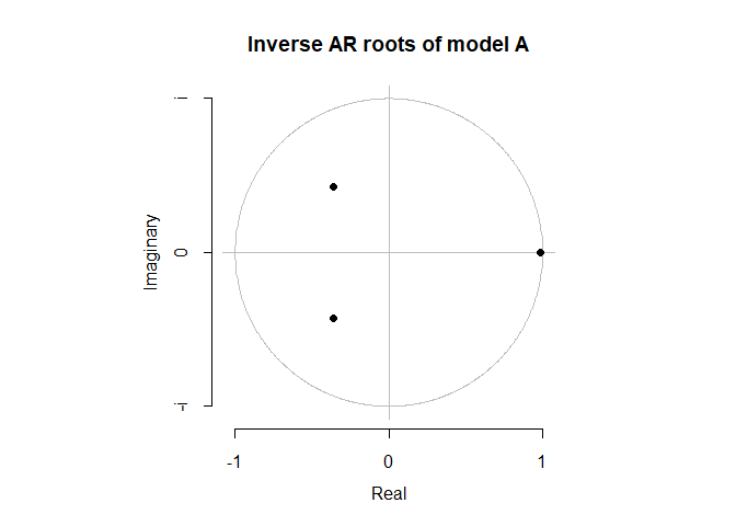
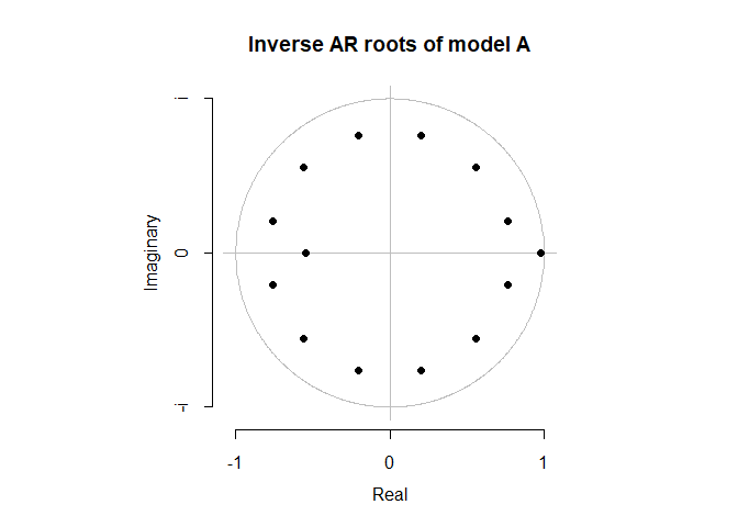
Before we move onto diagnostic checking, we want to make sure that our models are causal and stationary. Because model A and model D are both pure AR(p) models, they are always invertible. We show that both models are both causal and stationary because all of their roots lie inside of the unit circle.

Diagnostic Checking¶

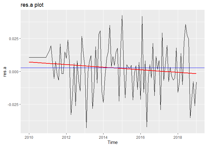
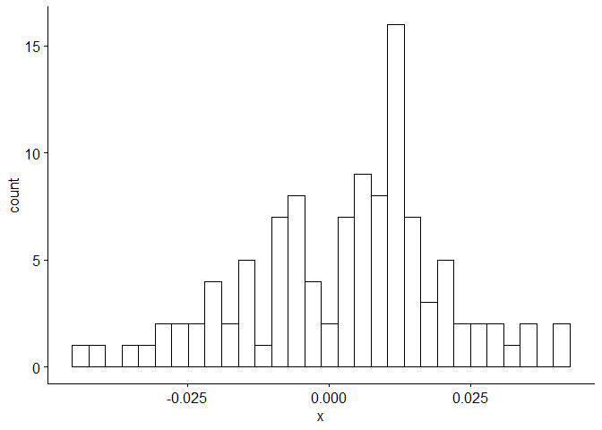
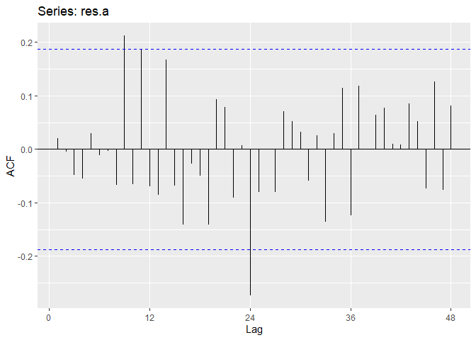
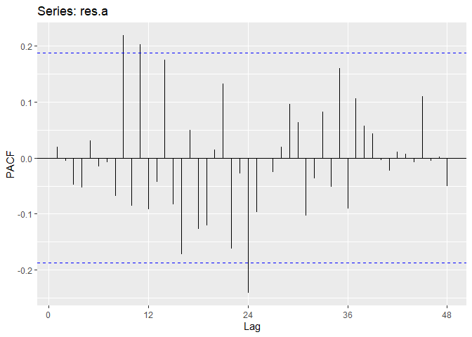
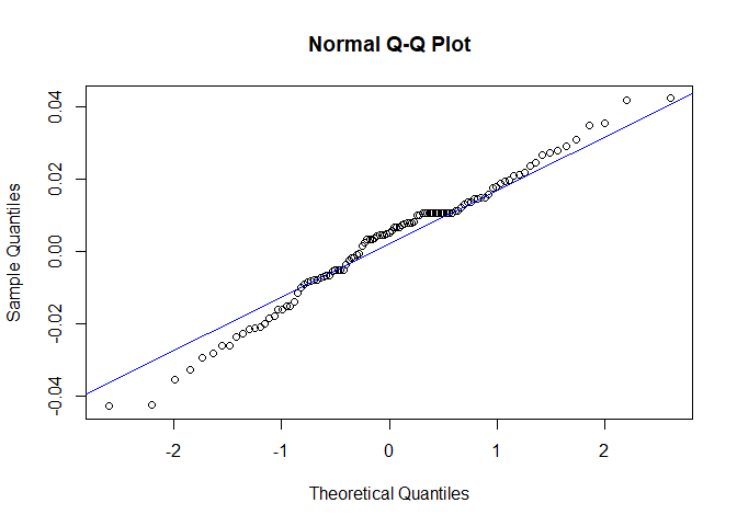
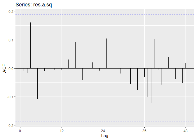
Now we will perform diagnostic checking on model A to determine whether our model is a good fit by analyzing the residuals. If our model is a good fit, the residuals should exhibit behavior similar to a White Noise process. Our plot of the residuals shows that the mean is about zero ,there is little to no trend, no seasonality, and no change in variance. The residuals are roughly normally distributed, and the quantile - quantile plot forms a straight line. The residuals also pass the Shapiro-Wilk normality test. The sample P/ACF of the residuals can be counted as 0 after applying Bartlett’s formula, as well as the ACF of the residuals squared. The residuals pass the Box-Pierce test and Ljung-Box test, so we accept our WN hypothesis at level 0.05. The squared residuals pass the Mcleod-li test so there is not nonlinear dependence. After applying Yule-Walker estimation and AICC statistics to the residuals, they come out as an AR(0) process so they are compatible with WN.

## 
##  Shapiro-Wilk normality test
## 
## data:  res.a
## W = 0.98174, p-value = 0.1409

## 
##  Box-Pierce test
## 
## data:  res.a
## X-squared = 10.395, df = 8, p-value = 0.2384

## 
##  Box-Ljung test
## 
## data:  res.a
## X-squared = 11.583, df = 8, p-value = 0.1708

## 
##  Box-Ljung test
## 
## data:  res.a.sq
## X-squared = 5.8357, df = 11, p-value = 0.8841

## 
## Call:
## ar(x = res.a, aic = TRUE, order.max = NULL, method = c("yule-walker"))
## 
## 
## Order selected 0  sigma^2 estimated as  0.0002988

## [1] "AICC of Model A"

## [1] -492.3585

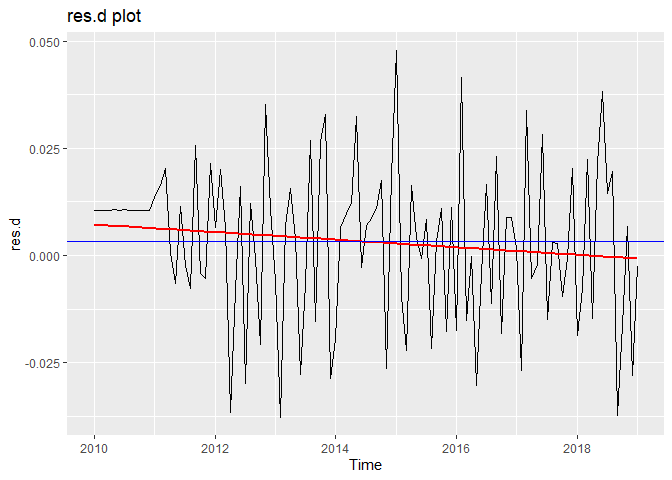
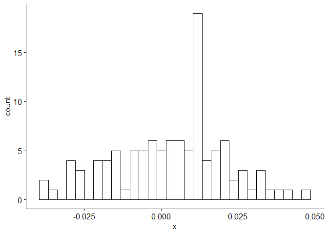
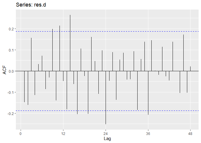
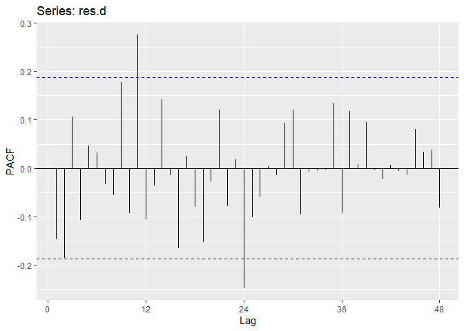
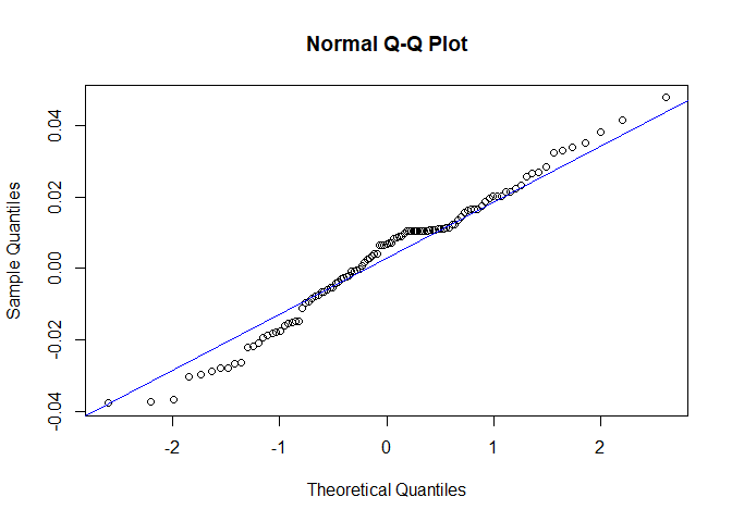
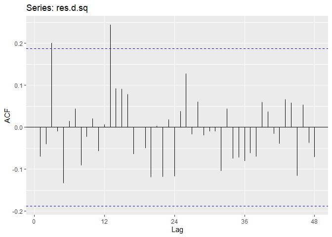
Now we perform diagnostic tests on model D. Our plot of the residuals shows that the mean is about zero ,there is little to no trend, no seasonality, and no change in variance. The residuals less normally distributed than model A, but the quantile - quantile plot still forms a straight line. The residuals pass the Shapiro-Wilk normality test. We see a few significant spikes in the P/ACF of the residuals, as well as the ACF of the residuals squared. The residuals fail the Box-Pierce test and Ljung-Box test, so we reject our WN hypothesis at level 0.05. The squared residuals pass the Mcleod-li test. After applying Yule-Walker estimation and AICC statistics to the residuals, they come out as an AR(2) process, showing that there is some information that is not being captured by our model. Based off the diagnostic checking, we reject model D as a good fit for the data.

## 
##  Shapiro-Wilk normality test
## 
## data:  res.d
## W = 0.98171, p-value = 0.1401

## 
##  Box-Pierce test
## 
## data:  res.d
## X-squared = 22.262, df = 9, p-value = 0.008085

## 
##  Box-Ljung test
## 
## data:  res.d
## X-squared = 24.164, df = 9, p-value = 0.00405

## 
##  Box-Ljung test
## 
## data:  res.d.sq
## X-squared = 9.2166, df = 11, p-value = 0.6019

## 
## Call:
## ar(x = res.d, aic = TRUE, order.max = NULL, method = c("yule-walker"))
## 
## Coefficients:
##       1        2  
## -0.1758  -0.1864  
## 
## Order selected 2  sigma^2 estimated as  0.000315

## [1] "AICC of Model D"

## [1] -484.6649

We choose model A because of the more desirable properties of its residuals and its lower AICc. Our final model is (1 − B¹²)(1 − 0.257B − 0.401B² − 0.313B³)X_t = Z_t

where Z_t ∼ N(0, 0.00032).

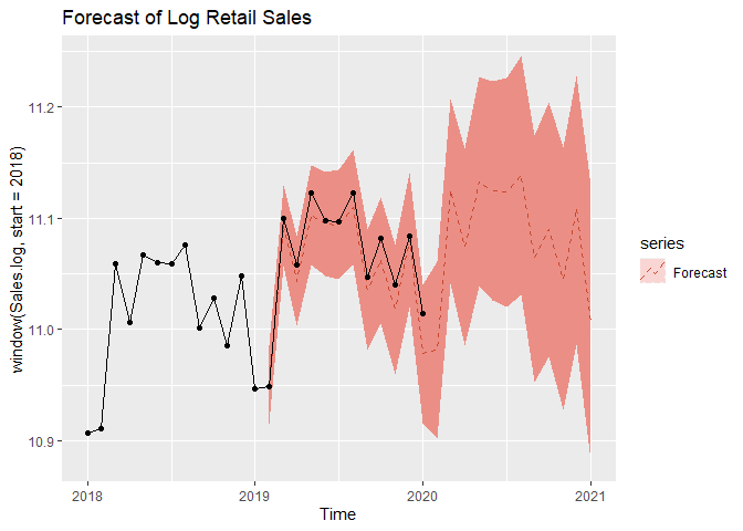
We now move on to forecasting. We assume an adequate time series model was obtained and MLE estimates of coefficents are obtained from the previous steps. We can forecast on the log-transformed data first. We can see that test set falls with our 95% Prediction intervals.

Forecasting¶

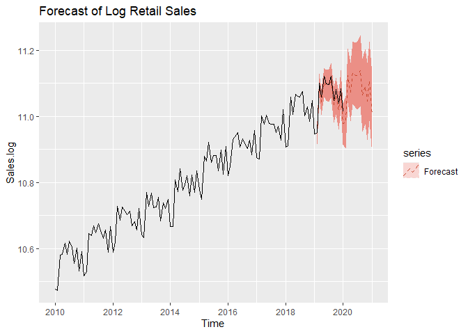
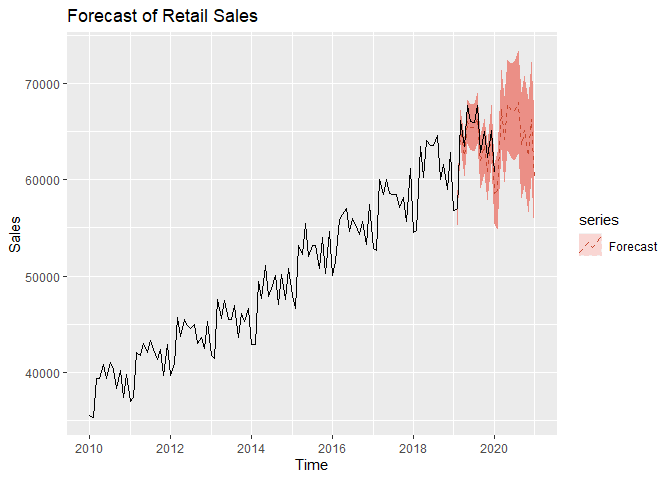
Now we forecast on the original data by exponentiating the forecasted values prior. The test set still falls within our 95% Prediction intervals.

IV. Conclusion¶

In conclusion, I was able to successfully model the data as a AR(3) process, differenced at lag 12 or as a SARIMA(3, 0, 0) × (0, 1, 0)₁₂. The final model was (1 − B¹²)(1 − 0.257B − 0.401B² − 0.313B³)X_t = Z_t

where Z_t ∼ N(0, 0.00032)

From our results we found that we could forecast retail sales in food services and drinking places that were close to the true values. We found that retail sales are generally the lowest in January, with the summer months of May to August being the busiest for this industry. There are spikes in activity in March, October, and December, coinciding with Spring break, Halloween, and Christmas. Our forecasts show a slow, steady growth in this industry over the next two years representing a safe investment opportunity. However, Covid-19 may cause permanent shifts in this industry, and the long-term effects of the pandemic are not captured in this study.

V. References¶

U.S. Census Bureau, Retail Sales [RSFSDPN], retrieved from FRED, Federal Reserve Bank of St. Louis; https://fred.stlouisfed.org/series/RSFSDPN, June 11, 2020.

VI. Appendix¶

# Convert data into time series object
Sales <- ts(Sales.csv[,2], start = c(2010,1),frequency=12)

# Split into Training/Test sets, leave 12 observations for forecasting
Sales.train <- ts(Sales[c(1:109)],start = c(2010,1),frequency=12)
Sales.test <- ts(Sales[c(110:length(Sales))],start = c(2019,2),frequency=12)

# Plot Training data with mean and trend
autoplot(Sales.train) +
  geom_smooth(method = "lm", se = FALSE, color = 'red') +             
  labs(x = "Year", y = "Millions of Dollars") +
  ggtitle("Sales.Train") +
  geom_hline(yintercept = mean(Sales), color="blue")

# Plot histogram of training data
gghistogram(Sales.train, add.normal=TRUE) # Data looks normally distributed

# Plot ACF
ggAcf(Sales.train, lag = 48) +
  ggtitle('ACF of Retail Sales')

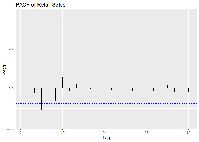
# Plot PACF
ggPacf(Sales.train, lag = 48) +
  ggtitle('PACF of Retail Sales')

## Boxcox transformation
bcTransform <- boxcox(Sales.train~as.numeric(1:length(Sales.train))) 
lambda = bcTransform$x[which(bcTransform$y == max(bcTransform$y))]
# lambda

# Since 0 is in confidence interval log transform data
Sales.train.log <- log(Sales.train)
Sales.log <- log(Sales)

# Plot log transformed Training data
autoplot(Sales.train.log) +
  labs(x = "Year", y = "Log Millions of Dollars") +
  ggtitle("Log Sales.train")

gghistogram(Sales.train.log, add.normal = TRUE) # Data looks normally distributed

# Plot ACF
ggAcf(Sales.train.log, lag = 48) +
  ggtitle('ACF of Log Retail Sales')

# Plot PACF
ggPacf(Sales.train.log, lag = 48) +
  ggtitle('PACF of Log Retail Sales')


## Differencing Sales.train.log at lag 12 to remove seasonality
print('Variance of Sales.train.log')
var(Sales.train.log)
Sales.train.log_12 <- diff(Sales.train.log, lag=12)
print('Variance of Sales.train.log differenced at lag 12')
var(Sales.train.log_12) # Variance is lower 
# var(Sales.train.log) > var(Sales.train.log_12)

# Plot
autoplot(Sales.train.log_12)+
  geom_smooth(method = "lm", se = FALSE, color = 'red') +
  geom_hline(yintercept = mean(Sales.train.log_12), color="blue") +
  labs(x = "Year", y = "Log Millions of Dollars") +
  ggtitle("Sales.train.log differenced at lag 12") 
# Data looks stationary after eliminating seasonality

gghistogram(Sales.train.log_12, add.normal=TRUE) # Data looks normally distributed

# Plot ACF 
ggAcf(Sales.train.log_12, lag = 100) +
  ggtitle('ACF of Log Retail Sales differenced at lag 12')

# Plot PACF
ggPacf(Sales.train.log_12, lag = 100) +
  ggtitle('PACF of Log Retail Sales differenced at lag 12')
  
# Differencing Sales.train.log again at lag 12 and lag 1 to remove trend

Sales.train.log_1_12 <- diff(Sales.train.log_12, lag=1)
print("Variance of Sales.train.log differenced at lag 1 and lag 12")
var(Sales.train.log_1_12) 

# var(Sales.train.log_12) > var(Sales.train.log_1_12) # Variance is higher, overdifferenced: Do not difference at lag 1

## Model Estimation
print("Model A")
# Estimate parameters of SARIMA model
a = arima(Sales.train.log, order=c(3,0,0), seasonal = list(order = c(0,1,0), period = 12),method="ML")
a

print("Model B")
# Estimate parameters of SARIMA model
b = arima(Sales.train.log, order=c(2,0,0), seasonal = list(order = c(1,1,0), period = 0), method="ML")
b

print("Model C")
# Estimate parameters of SARIMA model
c = arima(Sales.train.log, order=c(3,0,0), seasonal = list(order = c(1,1,0), period = 12), method="ML")
c

print("Model D")
# Estimate parameters of SARIMA model
d = arima(Sales.train.log, order=c(2,0,0), seasonal = list(order = c(0,1,0), period = 12), method="ML")
d

# Plot inverse roots of AR part: They should all be inside unit circle
plot(a, main = 'Inverse AR roots of model A')

# Plot inverse roots of AR part: They should all be inside unit circle
plot(b, main = 'Inverse AR roots of model A')


## Diagnostic Checking, model A
# Get residuals of model a
res.a <- residuals(a)

# Plot residuals
autoplot(res.a) +
  geom_smooth(method = "lm", se = FALSE, color = 'red') +   
  labs(x = "Time") +
  ggtitle("res.a plot") +
  geom_hline(yintercept = mean(res.a), color="blue")
# mean(res.a) # Sample mean is about 0

# Plot histogram of residuals
gghistogram(res.a,add.normal = TRUE)

# Plot ACF/PACF
ggAcf(res.a,lag.max = 48);ggPacf(res.a,lag.max=48)

# Normal Q-Q Plot
qqnorm(res.a) 
qqline(res.a,col='blue')

# square residuals for Mcleod-Li test
res.a.sq <- res.a^2
ggAcf(res.a.sq, lag.max = 48)

# Test residuals for normality
shapiro.test(res.a)

# Square-root of 121 = 11. p = 3, q = 0 so fitdf = p +q = 3
Box.test(res.a, lag=11, type = c('Box-Pierce'),fitdf =3) 
Box.test(res.a, lag=11, type = c('Ljung-Box'),fitdf =3)

# Mcleod-li test
Box.test(res.a.sq, lag=11, type = c('Ljung-Box'),fitdf =0)

# Check if residuals fit to WN Process
ar(res.a, aic = TRUE, order.max = NULL, method = c("yule-walker"))

print('AICC of Model A')
AICc(a)

## Diagnostic Checking, model D
# Get residuals of model c
res.d <- residuals(d)

# Plot residuals
autoplot(res.d) +
  geom_smooth(method = "lm", se = FALSE, color = 'red') +   
  labs(x = "Time") +
  ggtitle("res.d plot") +
  geom_hline(yintercept = mean(res.d), color="blue")
# mean(res.d) # Sample mean is about 0

# Plot histogram of residuals
gghistogram(res.d, add.normal = TRUE) 

# Plot ACF/PACF
ggAcf(res.d,lag.max = 48);ggPacf(res.d,lag.max=48)

# Normal Q-Q Plot
qqnorm(res.d) 
qqline(res.d,col='blue')

# square residuals for Mcleod-Li test
res.d.sq <- res.d^2
ggAcf(res.d.sq, lag.max = 48)

# Test residuals for normality
shapiro.test(res.d)

# Square-root of 121 = 11. p = 2, q = 0 so fitdf = p +q = 3
Box.test(res.d, lag=11, type = c('Box-Pierce'),fitdf =2)
Box.test(res.d, lag=11, type = c('Ljung-Box'),fitdf =2)

# Mcleod-li test
Box.test(res.d.sq, lag=11, type = c('Ljung-Box'),fitdf =0)

# Check if residuals fit to WN Process
ar(res.d, aic = TRUE, order.max = NULL, method = c("yule-walker"))

print('AICC of Model D')
AICc(d)

## Forecast on log-transformed data using Model A
autoplot(Sales.log, series = 'data',color='black') +
  autolayer(forecast(a,level=c(95)), series = 'Forecast',linetype='dashed') +
  autolayer(log(Sales.test), series='True values',color='black')+
  ggtitle('Forecast of Log Retail Sales')

# Zoom in
autoplot(window(Sales.log,start=2018), series = 'data',color='black') +
  autolayer(forecast(a,level=c(95)), series = 'Forecast', linetype='dashed') +
  autolayer(log(Sales.test), series='True values',color='black') +
  ggtitle('Forecast of Log Retail Sales') +
  geom_point()

# Fit model to and forecast original data
pred.orig <- forecast(arima(Sales.train, order=c(3,0,0), seasonal = list(order = c(1,1,0), period = 12),method="ML"),level=c(95))

## Forecast on original data using Model A
autoplot(Sales, series = 'data',color='black') +
  autolayer(pred.orig, series = 'Forecast', linetype='dashed') +
  autolayer(Sales.test, series='True values',color='black')+
  ggtitle('Forecast of Retail Sales')

# Zoom in
autoplot(window(Sales,start=2018), series = 'data',color='black') +
  autolayer(pred.orig,series = 'Forecast',  linetype='dashed') +
  ggtitle('Forecast of Retail Sales ') +
  autolayer(Sales.test, series='True values',color='black') + 
  geom_point() +
  ggtitle('Forecast of Retail Sales')

From school

League of Legends Win Classifier

Lawrence Lin